In this article, I’ll be taking you to a journey where we could view Variational Inference & ELBO in math perspective. A few concepts will be introduced but the detailed explainations of definition may be skipped to maintain a smooth and straight-forward logical flow. For those concepts, your favorite language model is your best thinking partner!
1. Vector Space & Notation Declarations
To ensure strict mathematical alignment, the following spaces and parameters are explicitly defined:
- $x \in \mathbb{R}^D$: Observed random vector (Data).
- $z \in \mathbb{R}^K$: Latent random vector.
- $\theta \in \mathbb{R}^M$: Generative model parameters (Decoder).
- $\phi \in \mathbb{R}^N$: Variational parameters (Encoder).
2. The Bottleneck of Bayesian Inference
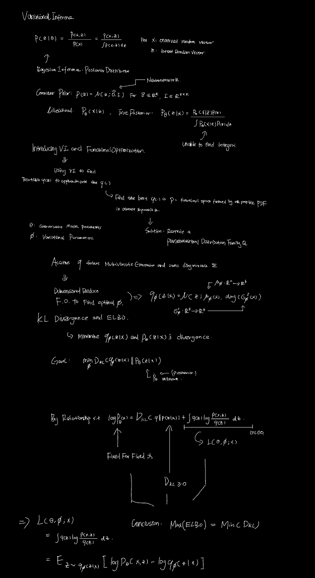
The objective of Bayesian inference is to compute the true posterior distribution:
$$p_\theta(z \mid x) = \frac{p_\theta(x \mid z)p(z)}{\int_{\mathbb{R}^K} p_\theta(x, z) dz}$$Problem: The denominator, Marginal Likelihood (Evidence) $p_\theta(x) = \int_{\mathbb{R}^K} p_\theta(x, z) dz$, requires integration over the high-dimensional latent space $\mathbb{R}^K$. For complex non-linear models (e.g., neural networks), this integral is analytically intractable.
3. Variational Inference (VI) & Parameterization
VI bypasses exact inference by transforming it into an optimization problem: approximate the intractable $p_\theta(z \mid x)$ with a tractable distribution $q(z \mid x)$.
- Functional Optimization Limitation: Finding the absolute optimal $q$ in the infinite-dimensional functional space of all valid PDFs is impossible.
- Parameterization: We restrict $q$ to a parameterized distribution family $\mathcal{Q}$ governed by $\phi$.
- Standard VAE Assumption:
- Prior: $p(z) = \mathcal{N}(z; \mathbf{0}, \mathbf{I})$
- Approximate Posterior: $q_\phi(z \mid x) = \mathcal{N}(z; \mu_\phi(x), \text{diag}(\sigma_\phi^2(x)))$
- (Note: $\mu_\phi: \mathbb{R}^D \to \mathbb{R}^K$ and $\sigma_\phi^2: \mathbb{R}^D \to \mathbb{R}^K$ are deterministic vector-valued functions parameterized by $\phi$.)
4. The Fundamental Identity (The Zero-Sum Game)
Our ultimate theoretical goal is to minimize the divergence between the approximation and the true posterior: $\min_{\phi} D_{KL}(q_\phi(z \mid x) \parallel p_\theta(z \mid x))$. By decomposing the log marginal likelihood, we obtain the fundamental identity:
$$\log p_\theta(x) = D_{KL}(q_\phi(z \mid x) \parallel p_\theta(z \mid x)) + \mathcal{L}(\theta, \phi; x)$$Where $\mathcal{L}(\theta, \phi; x) = \int_{\mathbb{R}^K} q_\phi(z \mid x) \log \frac{p_\theta(x, z)}{q_\phi(z \mid x)} dz$ is the Evidence Lower Bound (ELBO).
Core Mechanism:
- For a given observation $x$ and fixed generative parameters $\theta$, the term $\log p_\theta(x)$ is a strict constant.
- By Gibbs’ inequality, $D_{KL} \ge 0$, establishing $\log p_\theta(x) \ge \mathcal{L}(\theta, \phi; x)$.
- Due to the zero-sum constraint of the constant $\log p_\theta(x)$, maximizing the tractable ELBO $\mathcal{L}(\theta, \phi; x)$ w.r.t $\phi$ is mathematically strictly equivalent to minimizing the intractable $D_{KL}(q_\phi(z \mid x) \parallel p_\theta(z \mid x))$.
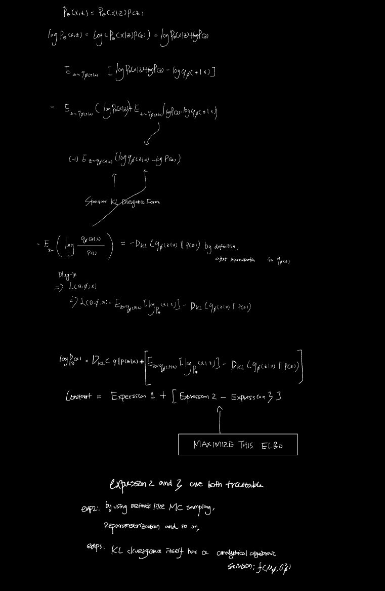
5. ELBO Decomposition & Analytical Extraction
Directly optimizing the integral form of the ELBO requires Monte Carlo sampling for the entire expression, resulting in exceptionally high gradient variance. We decompose the ELBO by applying the product rule $p_\theta(x, z) = p_\theta(x \mid z)p(z)$:
$$\mathcal{L}(\theta, \phi; x) = \underbrace{\mathbb{E}_{z \sim q_\phi(z \mid x)}[\log p_\theta(x \mid z)]}_{\text{Term 1: Reconstruction Error}} - \underbrace{D_{KL}(q_\phi(z \mid x) \parallel p(z))}_{\text{Term 2: KL Regularization Penalty}}$$Purpose of Decomposition:
- Term 1 still requires sampling (typically via the Reparameterization Trick) to estimate the expectation.
- Term 2 measures the divergence between two multivariate Gaussian distributions with diagonal covariance matrices. This specific topological constraint yields a strict closed-form analytical solution: $$D_{KL}(q_\phi(z \mid x) \parallel p(z)) = -\frac{1}{2} \sum_{j=1}^K \left( 1 + \log((\sigma_j)^2) - (\mu_j)^2 - (\sigma_j)^2 \right)$$ (where $\mu_j$ and $\sigma_j$ are the $j$-th scalar components of the vectors $\mu_\phi(x)$ and $\sigma_\phi(x)$).
By isolating Term 2 into an exact algebraic equation, we eliminate the need for stochastic sampling on this regularization penalty, drastically reducing the variance of the gradient estimators during backpropagation.
6. Handwritten Version
For those who prefer to see more straightforward logical structure or simply like handwritten stuff, here you go.